Learning Sampling Distribution in R Programming
Sampling distribution is the set of possible outcomes when we collect data through the randomization procedure (random sampling, ramond assignment). Do a simulation work is the best way to understand the sampling distribution. A simulation work is unrelated to any context we collect the data. You can connect the simulation work to any randominzation in the real world.
In this pseudo experiment, there are only ten observations we will collect in every sample. They are 1, 2, 3, 4, 5, 6, 7, 8, 9, 10. Accodring to the design of the experiment, a sample will have one observation to countless observations. I assume the distrubtions are accumulated from 100 samples of 1 observation, 9 observations, ,16 observations, 25 observations, and 36 observations. Every sample will be collapsed to a average value and become the components of sampling distribution. I use ggplot2 to draw the five sampling distributions. Look at what they are look like.
suppressPackageStartupMessages({
  library(ggplot2)
  library(xtable)
  })

set.seed(1)
OBV <- 1:10
Dist1 <- NULL
Dist9 <- NULL
Dist16 <- NULL
Dist25 <- NULL
Dist36 <- NULL
count = 100
while(count > 0){Dist1 <- c(Dist1,sample(OBV, 1, replace = TRUE)); count <- count - 1}
count = 100
while(count > 0){Dist9 <- c(Dist9,mean(sample(OBV, 9,replace = TRUE) ) ); count <- count - 1}
count = 100
while(count > 0){Dist16 <- c(Dist16,mean(sample(OBV, 16,replace = TRUE) ) ); count <- count - 1}
count = 100
while(count > 0){Dist25 <- c(Dist25,mean(sample(OBV, 25,replace = TRUE) ) ); count <- count - 1}
count = 100
while(count > 0){Dist36 <- c(Dist36,mean(sample(OBV, 36,replace = TRUE) ) ); count <- count - 1}
Dist.df <- data.frame(Size = factor(rep(c(1,9,16,25,36), each=100)), Sample_Means = c(Dist1, Dist9, Dist16, Dist25, Dist36) )
ggplot(Dist.df, aes(Sample_Means, fill = Size)) + geom_histogram() + facet_grid(. ~ Size)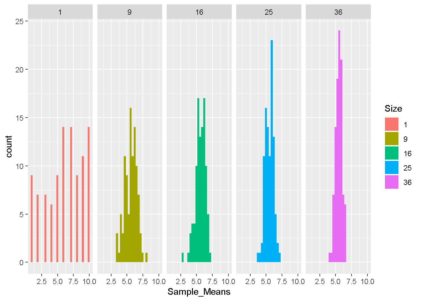
We call the set of observations 1, 2, 3, 4, 5, 6, 7, 8, 9, 10 population in any circumstance we conduct this experiment. This population has the average 5.5 and the variance/standard deviation 8.25/2.87. With the increase of sample size, you find more and more samples collapsed to the average of population. The variation of each sample distribution decreases with the increasing of sample size as well. The following table illustrate the average and variance/standard deviation of each sampling distribution.
| Sample Size | Average | Variance | Standard Deviation |
|---|---|---|---|
| 1 | 6.06 | 8.14 | 2.85 |
| 9 | 5.62 | 0.91 | 0.96 |
| 16 | 5.6 | 0.58 | 0.76 |
| 25 | 5.54 | 0.43 | 0.66 |
| 36 | 5.51 | 0.27 | 0.52 |
There are three findings in this simulation. First, the average of every sample is as equal as the average of population. Second, the variance of every sample is close to the divide of population variance by the sample size. Third, the standard deviation of every sample is close to the divide of population standard deviation by the square of sample size. These facts matches Central limit theorem.
!登入個人github帳號就能留言!